population <- read_csv("https://info3370.github.io/data/baseball_with_record.csv")Statistical Learning
The reading with this class is Berk 2020 Ch 1 p. 1–5, stopping at paragraph ending “…is nonlinear.” Then p. 14–17 “Model misspecification…” through “…will always be in play.”
Statistical learning is a term that captures a broad set of ideas in statistics and machine learning. This page focuses on one sense of statistical learning: using data on a sample to learn a subgroup mean in the population.
As an example, we continue to use the data on baseball salaries, with a small twist. The file baseball_with_record.csv contains the following variables
playeris the player nameteamis the team namesalaryis the 2023 salaryrecordis the 2022 proportion of games won by that teamtarget_subgroupis codedTRUEfor the L.A. Dodgers andFALSEfor all others
Our goal: using a sample, estimate the mean salary of all Dodger players in 2023. Because we have the population, we know the true mean is $6.23m.
A sparse sample will hinder our ability to accomplish the goal. We will work with samples containing many MLB players, but only a few Dodgers. We will use statistical learning strategies to pool information from those other teams’ players to help us make a better estimate of the Dodger mean salary.
Our predictor will be the record from the previous year. We assume that teams with similar win percentages in 2022 might have similar salaries in 2023.
Prepare our data environment
For illustration, draw a sample of 5 players per team
sample <- population |>
  group_by(team) |>
  sample_n(5) |>
  ungroup()
Construct a tibble with the observation to be predicted: the Dodgers.
to_predict <- population |>
  filter(target_subgroup) |>
  distinct(team, record)
Ordinary least squares
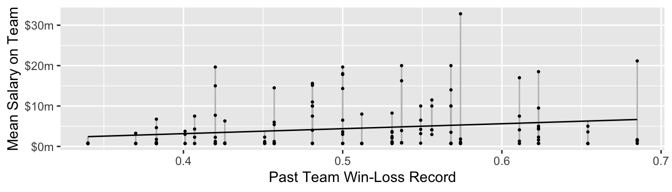
We could model salary next year as a linear function of team record by Ordinary Least Squares. In math, OLS produces a prediction \[\hat{Y}_i = \hat\alpha + \hat\beta X_i\] with \(\hat\alpha\) and \(\hat\beta\) chosen to minimize the sum of squared errors, \(\sum_{i=1}^n \left(Y_i - \hat{Y}_i\right)^2\). Visually, it minimizes all the line segments below.
Here is how to estimate an OLS model using R.
model <- lm(salary ~ record, data = sample)Then we could predict the mean salary for the Dodgers.
to_predict |>
  mutate(predicted = predict(model, newdata = to_predict))
# A tibble: 1 × 3
team record predicted
<chr> <dbl> <dbl>
1 L.A. Dodgers 0.685 6668053.Our model-based estimate compares to the true population mean of $6.23m.
Penalized regression
Penalized regression is just like OLS, except that it prefers coefficient estimates that are closer to 0. This can reduce sampling variability. One penalized regression is ridge regression, which penalizes the sum of squared coefficients. In our example, it estimates the parameters to minimize
\[\underbrace{\sum_{i=1}^n \left(Y_i - \hat{Y}_i\right)^2}_\text{Squared Error} + \underbrace{\lambda\beta^2}_\text{Penalty}\]
where the positive scalar penalty \(\lambda\) encodes our preference for coefficients to be near zero. Otherwise, penalized regression is just like OLS!
The gam() function in the mgcv package will allow you to fit a ridge regression as follows.
library(mgcv)model <- gam(
salary ~ s(record, bs = "re"),
data = sample
)Predict the Dodger mean salary just as before,
to_predict |>
  mutate(predicted = predict(model, newdata = to_predict))
# A tibble: 1 × 3
team record predicted
<chr> <dbl> <dbl[1d]>
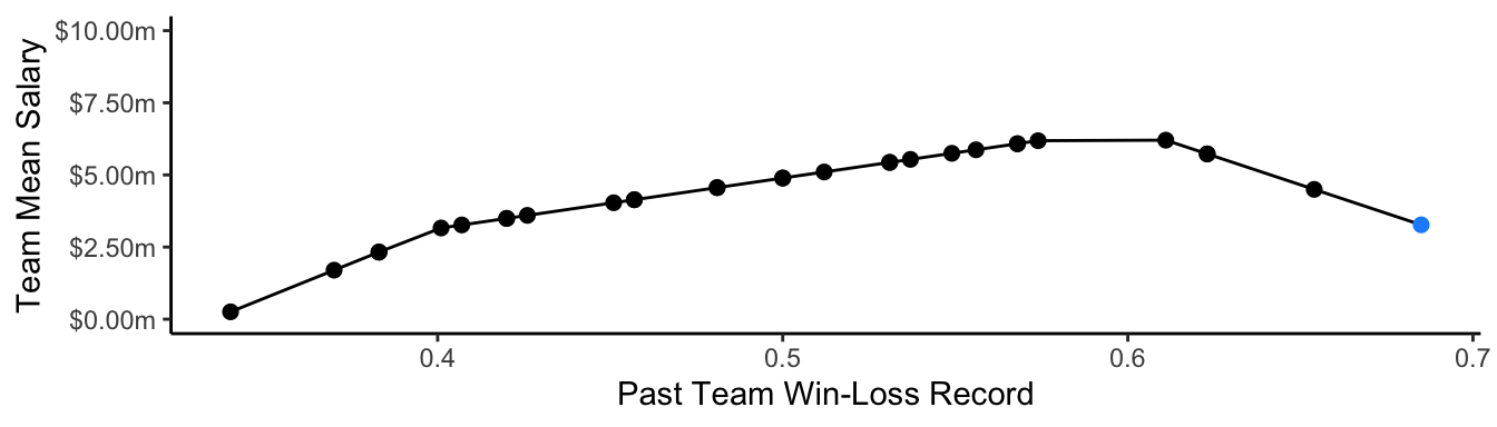
1 L.A. Dodgers 0.685 6252449.Splines
We may want to allow a nonlinear relationship between the predictor and the outcome. One way to do that is with splines, which estimate part of the model locally within regions of the predictor space separated by knots. The code below uses a linear spline with knots at 0.4 and 0.6.
library(splines)
model <- lm(
  salary ~ bs(record, degree = 1, knots = c(.4,.6)),
  data = sample
)
We can predict the Dodger mean salary just as before!
to_predict |>
  mutate(predicted = predict(model, newdata = to_predict))
# A tibble: 1 × 3
team record predicted
<chr> <dbl> <dbl>
1 L.A. Dodgers 0.685 3269869.Trees
Perhaps our response surface is bumpy, and poorly approximated by a smooth function. Decision trees search the predictor space for discrete places where the outcome changes, and assume that the response is flat within those regions.
library(rpart)
model <- rpart(salary ~ record, data = sample)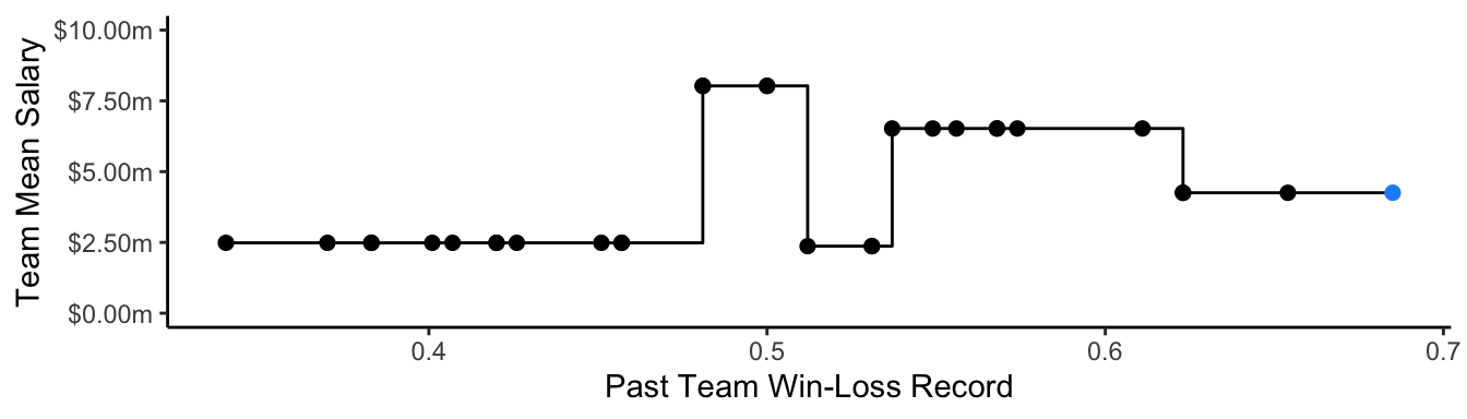
Predict as in the other strategies.
to_predict |>
  mutate(predicted = predict(model, newdata = to_predict))
# A tibble: 1 × 3
team record predicted
<chr> <dbl> <dbl>
1 L.A. Dodgers 0.685 4253845.Conclusion
Statistical learning in this framing is all about
- we have a subgroup with few sampled units (the Dodgers)
- we want to use other units to help us learn
- our goal is to predict the population mean in the subgroup