library(tidyverse)Visualization
Prerequisites. You should first install R and RStudio as described in the R4DS Prerequisites. If you are unfamiliar with the layout of RStudio, see the User Guide.
In this discussion section, we will
- load the data from Jencks 2002 Table 1
- visualize the data using
ggplot
Getting started
In your table groups, introduce yourselves
- what made you interested in this class
- how much experience do you have with R and
ggplot?
Whoever has the least experience—you are the coder! Arrange yourselves so that everyone can see the coder’s screen.
Prepare the environment
Open a new R Script by clicking the button at the top left of RStudio. Save your R Script in a folder you will use for this exercise.
Paste the code below into your R Script. Place your cursor within the line and hit CMD + Enter or CTRL + Enter to run the code and load the tidyverse package.
You will see action in the console. You have added some functionality to R for this session!
The data can be loaded from the course website with the line below.
data <- read_csv(file = "https://info3370.github.io/data/jencks_table1.csv")When you run this code, the object data will appear in your environment pane.
Explore the data
Type data in your console. You can see the data!
countrycountry nameratioratio of 90th to 10th percentile of household income. You can think of this as how many dollars a high-income household receives for each dollar that a low-income household receivesgdpGross Domestic Product Per Capita, expressed as a proportion of U.S. GDPlife_expectancylife expectancy at birth
For details on the data, see Jencks (2002) Table 1.
Produce a graph
We are ready to produce a graph! The code below will produce a simple graph.
data |>
  ggplot(mapping = aes(x = ratio, y = gdp)) +
  geom_point()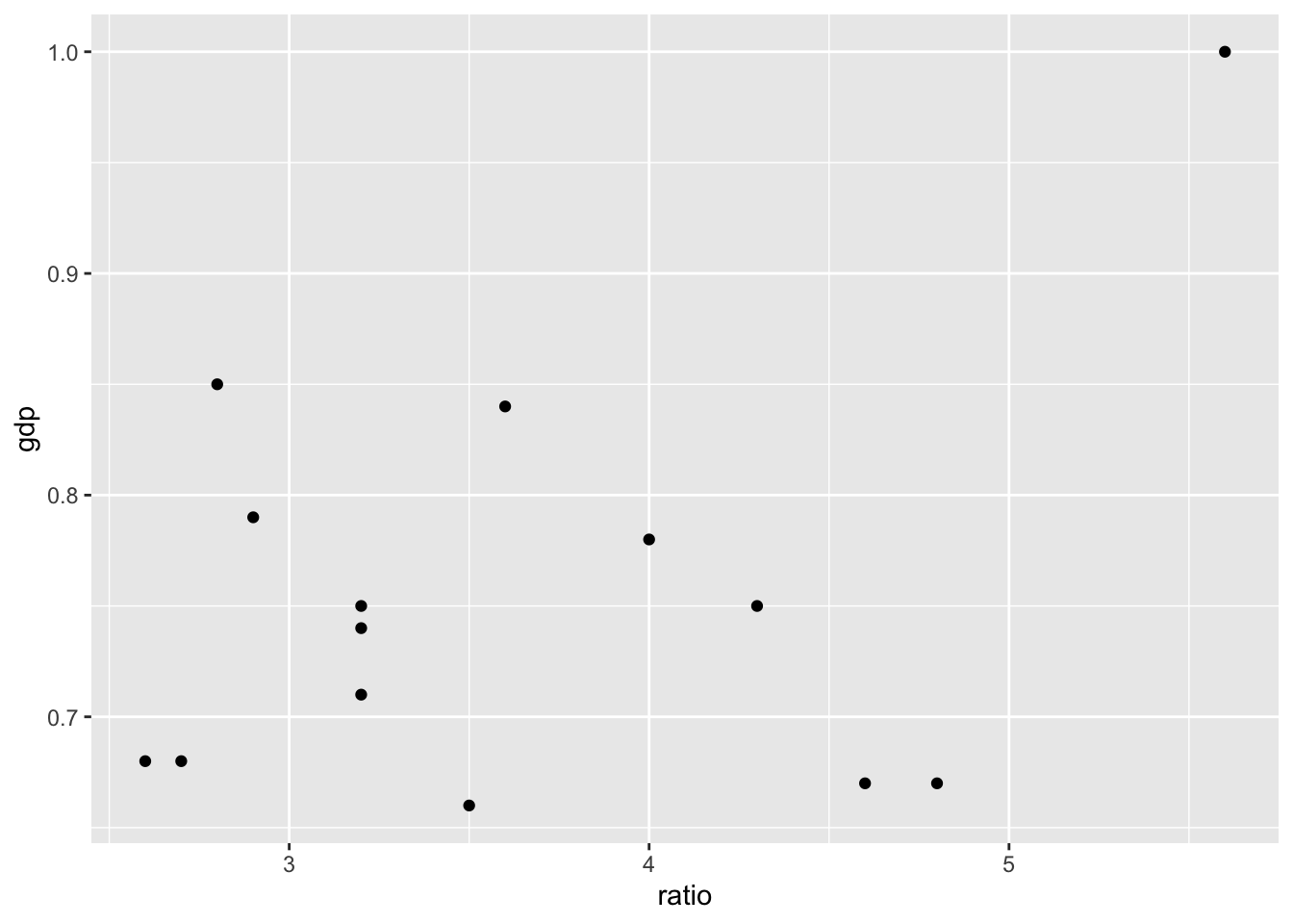
Let’s break this code down into pieces
datatells R to start with the objectdata|>is called the pipe operator. It passes thedataobject down to the function in the next lineggplot()is a function that creates a plot environment- the argument
mapping = aes(x = ratio, y = gdp)tellsggplot()how variables in the data will correspond to elements of the plot. We will visualizeratioon the x-axis andgdpon the y-axis +tellsggplot()we will add a new layer on the next linegeom_point()tellsggplot()to add a layer of points to the graph
Customizing your graph
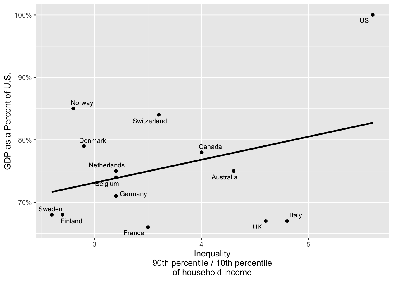
In your group, create additional layers with additional lines connected by +. Be creative! Here are some ideas:
- label the axes with
scale_x_continuous(name = "your text here")andscale_y_continuous(name = "your text here") - label countries using
geom_textorgeom_text_repel, with the aestheticlabel = country
There are many possible graphs to make. An example is below.
Interpret your graph
Once you are happy with your graph,
- write a few sentences explaining your graph
- discuss what questions you would like to ask next
Prepare a Quarto report
Create a new Quarto document. Put your R code and interpretation into that document. Upload to Canvas!