Class

Social class is a concept with many definitions: ownership of capital, position within the power relations of economic production, ways of being that are tied to one’s upbringing, etc. We will not cover class in depth. With a few examples, we will discuss some ways to study class using data science.

The structure of this page is first material for discussion, then material for the corresponding lecture which followed discussion.

Exercise: Subjective class identifications

How do people think about social class? In repeated surveys back to 1972, the General Social Survey has asked respondents:

If you were asked to use one of four names for your social class, which would you say you belong in: the lower class, the working class, the middle class, or the upper class?

How would you answer this question? How do you think most Americans would answer it?

In discussion, we will work with a prepared dataset that contains the answers to this question and a few others. You can see the documentation to see what the values mean in the GSS Data Explorer. You also might find other variables there to use in your final project! See the video below for an intro to the GSS.

To jump straight into our prepared data file, run this line of code.

gss <- read_csv("https://info3370.github.io/data/gss.csv")

The data contain a series of variables. Our exercise will focus on the following, each of which links to the documentation.

wtssall is the survey weight
class is the answer to the survey question above
padeg and madeg are the highest degree attained by the respondent’s father and mother, respectively
degree is the respondent’s highest degree attained
age is the respondent’s age at the time of the survey

We will use these data to estimate:

the distribution of subjective social class among Americans age 25+
how that varies across those with and without a college degree
and across the four subgroups defined by the respondent’s degree and whether at least one of the respondent’s parents had a college degree

The code below helps with some data preparation steps to get you started.

Restrict the sample

We want to restrict to our target population, and to those with valid responses on the relevant variables. We want to report the number of cases remaining after each restriction, in the interest of transparency. Here is a custom function that can be included in your piped sequence to report the sample size.

print_rows <- function(.data, comment = "cases remain") {
  print(paste(prettyNum(nrow(.data), big.mark = ","), comment))
  return(.data)
}

As with all canned functions like mutate and summarize, the first argument is the dataset. The second argument is a comment to say why a restriction occurred. The function prints the comment and the number of cases that remain. Then, it returns the dataset unchanged.

There are many ways to track sample restrictions—this is just one custom way! Below is code that restricts our data and reports sample sizes using this function.

gss_restricted <- gss |>
  filter(wtssall > 0) |>
  print_rows(comment = "have positive weights") |>
  filter(padeg >= 0 & madeg >= 0) |>
  print_rows(comment = "are age 25+") |>
  filter(age >= 25) |>
  print_rows(comment = "have valid parents' degree") |>
  filter(degree >= 0) |>
  print_rows(comment = "have valid own degree") |>
  filter(class %in% 1:4) |>
  print_rows(comment = "have valid own subjective class")

[1] "64,814 have positive weights"
[1] "45,815 are age 25+"
[1] "41,141 have valid parents' degree"
[1] "41,076 have valid own degree"
[1] "39,878 have valid own subjective class"

Prepare the variables

The variables as downloaded are coded in numbers. The code below converts them to intuitive labels.

parent_college will be a logical variable coded TRUE if at least one parent finished a four-year degree and FALSE otherwise
respondent_college will be a logical variable coded TRUE if the respondent finished a four-year degree and FALSE otherwise
class will be recoded to be a factor variable with character labels

gss_prepared <- gss_restricted |>
  mutate(
    parent_college = padeg >= 3 | madeg >= 3,
    respondent_college = degree >= 3,
    class = factor(class, labels = c("Lower class","Working class","Middle class","Upper class"))
  ) |>
  select(parent_college, respondent_college, class, wtssall)

Produce visualizations

Now answer the questions that motivated this data analysis:

what is the distribution of self-identified social class?
what is the distribution among those with and without a degree?
what is the distribution in (2) further subdivided by whether at least one parent held a degree?

Worked answers to discussion activity

The code below summarizes the distribution self-identified social class.

gss |>
  # drop cases with invalid outcome or negative weight
  filter(class > 0 & class < 5 & wtssall > 0) |>
  # calculate total weight within each class
  group_by(class) |>
  summarize(prop = sum(wtssall), .groups = "drop") |>
  # convert to proportion of total across all classes
  mutate(prop = prop / sum(prop)) |>
  ggplot(aes(x = class, y = prop)) +
  geom_bar(stat = "identity") +
  geom_text(aes(y = .005, label = scales::label_percent(accuracy = 1)(prop)), color = "white",
            vjust = 0) +
  scale_x_continuous(
    breaks = 1:4,
    labels = c("Lower\nClass","Working\nClass","Middle\nClass","Upper\nClass")
  ) +
  ylab("Proportion Identifying with Each Class") +
  xlab("Class")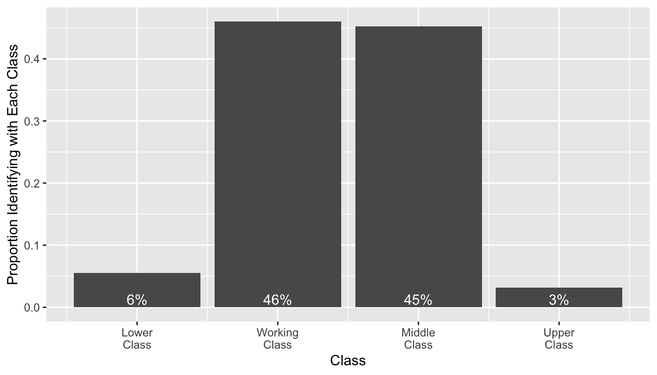

The code below summarizes the distribution self-identified social class among those with and without a college degree.

gss |>
  # drop cases with invalid outcome, predictor, or negative weight
  filter(class > 0 & class < 5) |>
  filter(degree %in% 0:4) |>
  filter(wtssall > 0) |>
  # create indicator of collge degree
  # see codes at https://gssdataexplorer.norc.org/variables/59/vshow
  mutate(college = case_when(
    degree %in% 3:4 ~ "Holds a Four-Year Degree",
    degree %in% 0:2 ~ "No Four-Year Degree",
  )) |>
  # calculate total weight within each class
  group_by(college, class) |>
  summarize(prop = sum(wtssall), .groups = "drop_last") |>
  # convert to proportion of total across all classes within college degrees
  group_by(college) |>
  mutate(prop = prop / sum(prop)) |>
  ggplot(aes(x = class, y = prop)) +
  facet_wrap(~college) +
  geom_bar(stat = "identity") +
  geom_text(aes(label = scales::label_percent(accuracy = 1)(prop)),
            vjust = -.2) +
  scale_x_continuous(
    breaks = 1:4,
    labels = c("Lower\nClass","Working\nClass","Middle\nClass","Upper\nClass")
  ) +
  ylab("Proportion Identifying with Each Class") +
  ylim(c(0,1)) +
  xlab("Class")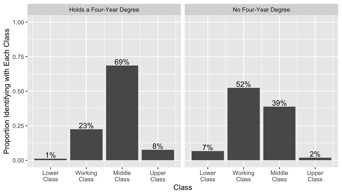

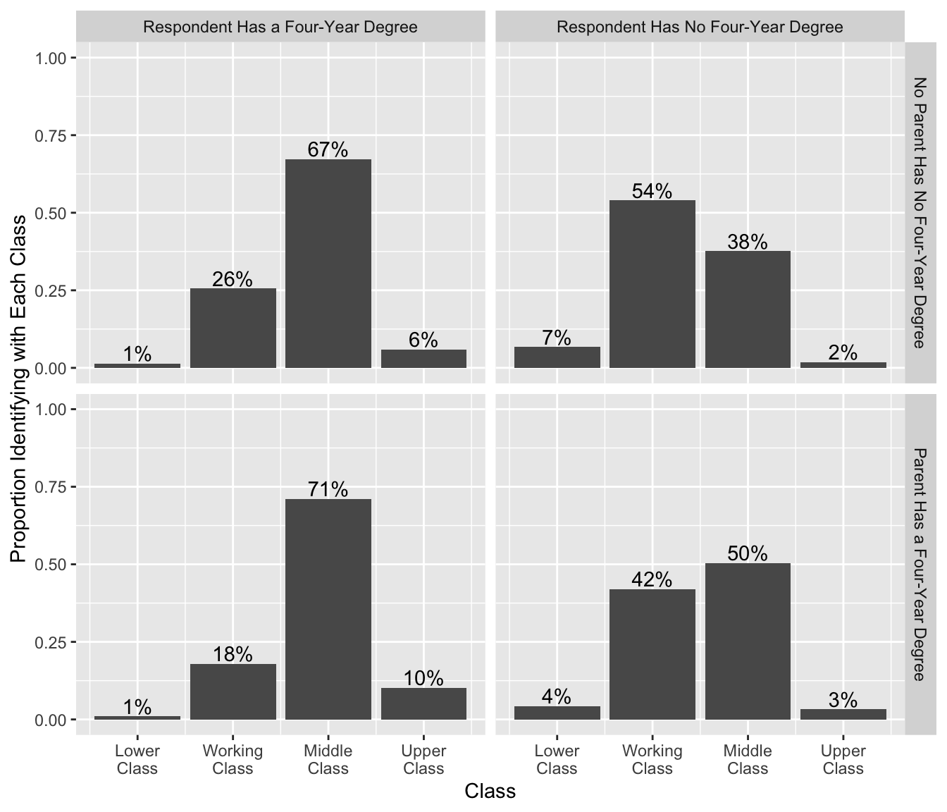
The code below summarizes the class distribution by own and parents’ degree attainment.

gss |>
  # drop cases with invalid outcome, predictor, or negative weight
  filter(class > 0 & class < 5) |>
  filter(degree %in% 0:4) |>
  filter(padeg %in% 0:4 | madeg %in% 0:4) |>
  filter(wtssall > 0) |>
  # create indicator of collge degree
  # see codes at https://gssdataexplorer.norc.org/variables/59/vshow
  mutate(child_college = case_when(
    degree %in% 3:4 ~ "Respondent Has a Four-Year Degree",
    degree %in% 0:2 ~ "Respondent Has No Four-Year Degree",
  )) |>
  mutate(parent_college = case_when(
    padeg %in% 3:4 | madeg %in% 3:4 ~ "Parent Has a Four-Year Degree",
    T ~ "No Parent Has No Four-Year Degree",
  )) |>
  # calculate total weight within each class
  group_by(parent_college, child_college, class) |>
  summarize(prop = sum(wtssall), .groups = "drop_last") |>
  # convert to proportion of total across all classes within college degrees
  group_by(parent_college, child_college) |>
  mutate(prop = prop / sum(prop)) |>
  ggplot(aes(x = class, y = prop)) +
  facet_grid(parent_college ~ child_college) +
  geom_bar(stat = "identity") +
  geom_text(aes(label = scales::label_percent(accuracy = 1)(prop)),
            vjust = -.2) +
  scale_x_continuous(
    breaks = 1:4,
    labels = c("Lower\nClass","Working\nClass","Middle\nClass","Upper\nClass")
  ) +
  ylab("Proportion Identifying with Each Class") +
  ylim(c(0,1)) +
  xlab("Class")

Exercise: Subjective class identifications

Restrict the sample

Prepare the variables

Produce visualizations

Worked answers to discussion activity

Lecture: Social class