Machine learning: Interactive nonlinearity via random forest with grf
Perhaps we think that predictors may interact: the response to one predictor differs greatly as a function of the values of the other predictor. Random forests are a method that can discover interactions in data.
The grf package supports this type of estimation. Start by preparing the environment.
library(tidyverse)
library(grf)
learning <- read_csv("learning.csv")
holdout_public <- read_csv("holdout_public.csv")
The base of a random forest: Decision trees
To understand a random forest, you first need to understand a decision tree. Below is a decision tree applied to our data.
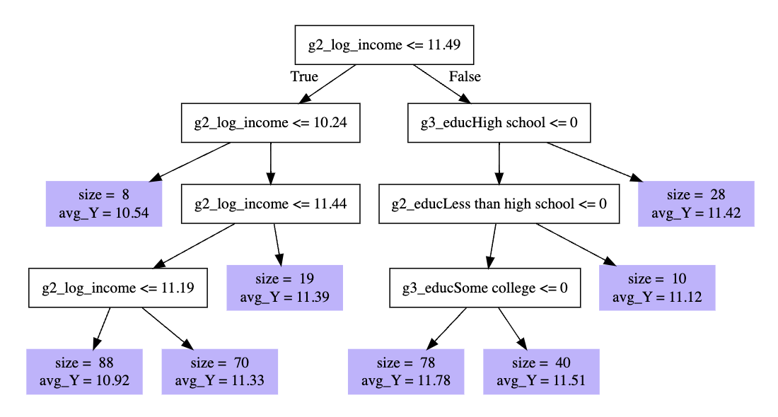
What happened there? A high level take
- the algorithm looked over all predictors and values to find a split that would reduce mean squared prediction error
- it first split into those with
g2_log_income <= 11.49and everyone else - within each subgroup, it then found another useful split
- it continued down the branches of the tree to the leaves (purple)
Each leaf is an interactive function of predictors.
Example: At the far right is a leaf with 28 observations who have
g2_log_income > 11.49and whose grandparents’ education is not equal to high school.
For a new case, we would drop it down the branches until we landed in a leaf. The prediction is the average outcome of the training cases who also landed in that leaf.
From trees to a forest
A random forest is an ensemble of trees. Repeatedly, the algorithm samples cases and samples variables. For each repetition, it grows a tree. The prediction from the forest is the average over many trees. The key advantage of a forest is that the predictions are more stable (less sensitive to perturbations to the sample) than are individual trees.
Using grf to learn a forest
The code below estimates a forest using the grf package.
library(grf)
First, define a formula of predictors
formula_of_predictors <- formula(~ -1 + race + sex +
                                   g1_educ + g2_educ + g3_educ +
                                   g1_log_income + g2_log_income)
Then, create a matrix of predictors in the learning and holdout sets.
X_learning <- model.matrix(formula_of_predictors,
                           data = learning)
X_holdout <- model.matrix(formula_of_predictors,
                          data = holdout_public)
Define the outcome in the learning set.
y_learning <- learning$g3_log_income
Fit the forest
fit <- regression_forest(X = X_learning,
                         Y = y_learning,
                         tune.parameters = "all")
Make predictions for the holdout set
fitted.grf <- predict(fit,
                      newdata = X_holdout)
fitted <- holdout_public %>%
  mutate(g3_log_income = fitted.grf$predictions)
To learn more, I would recommend
- Tibshirani et al. Generalized Random Forest. Software website with tutorials.
- Athey, Tibshirani, and Wager. 2019. Generalized random forests. Annals of Statistics 47(2):1148-1178.