Problem Set 4. Intervening to Equalize Opportunity

Info 3370. Studying Social Inequality with Data Science. Spring 2023

Due: 5pm on 21 Apr 2023. Submit on Canvas.

After grades are released: If you think you have been graded in error, we will only consider regrade requests submitted here. All requests must be submitted within 72 hours of grade release.

Welcome to the fourth problem set! This problem set is about causal inference methods to study an intervention (a college degree) that might help to equalize economic opportunity.

• Before you begin, you download and unzip pset4.zip. This contains several files that will be put in one working directory. Use the included .Rmd to complete the assignment
• In Canvas, you will upload the PDF produced by your .Rmd file
• Don’t put your name on the problem set. We want anonymous grading to be possible
• We’re here to help! Reach out using Ed Discussion or office hours

The header of this problem set has a few steps to get you set up, which we have streamlined as much as possible so you can focus on the causal problems.

Data access

This problem set uses data from the National Longitudinal Survey of Youth 1997 (NLSY97). The NLSY97 began with a probability sample of U.S. non-institutionalized youths ages 12–17 in 1997, and has followed them in repeated interviews through 2019.

To access data, you will

1. Visit the NLS Investigator and register for an account
2. Log in. Choose the NLSY97 study and the substudy “NLSY97 1997–2019 (rounds 1–19).”
3. Under “Choose Tagsets”, find where it says “Upload Tagset.” Click “Choose File” and upload our tagset: pset4.NLSY97, which is part of the zipped folder you downloaded for this problem set. This will load the variables we will use into your session.
4. Click “Save/Download” -> “Advanced Download”. Check the box for “R Source code” and any other boxes you want. In the filename box, type “pset4” and click “Download.”
5. Move the downloaded file pset4.dat into the unzipped folder you downloaded for this problem set

Note: The file you download will be under 200KB.

Data preparation

You’ve done data preparation in previous homework, so we don’t want that to take your time now. We made some code to help. Put your downloaded pset4.dat file in the directory where this .Rmd is located. The code below will prepare a data file for you.

library(tidyverse)
source("pset4_prep.R")

The resulting data file d contains several variables:

• respondent_college is our treatment. It indicates whether the respondent completed a four-year college degree
• fulltime_2019 is the outcome variable, which indicates whether the respondent was employed at least 30 hours per week at the time of the 2019 interview
• sex coded Female and Mle
• race coded Black, Hispanic, White / Other
• parent_college indicates whether the respondent’s parent completed college
• mom_age_at_birth is the respondent’s mother’s age at the birth of the respondent
• children_under_18 is the number of children under 18 in the respondent’s household in the 1997 survey
• two_parent_household indicates whether the parent lived with two residential parents in 1997, where parent is defined to include non-biological residential parents
• region is coded in four U.S. regions for residence in 1997
• urban indicates residence in an urban area in 1997
• income_1997 is gross household income in 1997

Part 1 (10 points). Nonparametric estimation

We will estimate the causal effect of the respondent completing college on whether that respondent works full-time in the 2019 interview. To practice nonparametric estimation, we will assume at first that the only confounder is whether the parent completed collge.

• Estimate the causal effect of respondent_college on fulltime_2019 by conducting analysis within subgroups defined by parent_college
• Report the conditional average causal effect in each of these two subgroups (a printout from R is fine)

# your code here

Part 2 (25 points). Parametric estimation with logistic regression

2.1 (4 points). Estimate a statistical model

Estimate a logistic regression model (a glm() with family = binomial) predicting full-time employment in 2019. For your model formula, interact respondent_college with an additive function of all confounders.

Hint: You could use the model formula fulltime_2019 ~ respondent_college*(.), where the . tells R to include all the variables there.

# your code here

2.2 (5 points). Predict potential outcomes

Create data frames with counterfactual treatment values of interest: respondent_college = TRUE and respondent_college = FALSE.

# your code here

Predict the potential outcome under each treatment condition, and difference to estimate the conditional average causal effect at the confounder values of each respondent.

# your code here

2.3 (4 points). Average effect by parent_college

Report the conditional average effect within subgroups defined by parent_college. A printout is fine. Interpret the two estimates in a sentence written so that a parent reading the Cornell Daily Sun could understand.

# your code here

Your interpretation here.

2.4 (4 points) Histogram of conditional average effects

Create a histogram (geom_histogram()) showing the full distribution of estimated conditional average causal effects. Interpret in a sentence that a parent reading the Cornell Daily Sun could understand.

# your code here

Your interpretation here.

2.5 (4 points) Scatterplot of conditional average effects

Create a scatterplot with income_1997 on the $x$-axis and the estimated conditional average causal effect on the $y$-axis. Someone might expect these points to fall all on a single curve. Why don’t they? In other words, why do effects vary among those with the same family income?

# your code here

2.6 (4 points) Your choice

Choose some other confounding variable. Visualize how the conditional average causal effect of college varies as a function of that variable.

Part 3 (15 points). Summarizing the big ideas.

On Canvas under “Files”, you will find a PDF draft of a forthcoming book that we have permission to read internally as a class but not share more broadly.

Brand, Jennie E. 2023. Overcoming the Odds: The Benefits of Completing College for Unlikely College Graduates. New York: Russell Sage Foundation.

The ideas in this book have inspired much of this problem set. Read the following selections. Note that pages are internally numbered within each chapter.

• Ch 1 p. 2-7 (the intro to the book)
• Ch 3 p. 1-6 (intro to chapter 3 and the section “Counterfactuals and potential outcomes”)
• Ch 3 p. 19-23 (the section “Identifying effects of college completion”)

Consider our discussions in class and the ideas in this reading. In a paragraph written to someone who knows nothing about causal inference, explain

• What is the college counterfactual? Why is it so helpful to think this way, as opposed to in comparisons across people who go to college and those who do not? Try to explain as though writing to someone who has neither read the book nor studied causal inference.
• What makes the search for effect heterogeneity particularly worthwhile when research may inform policy about college access?

Your answer here.

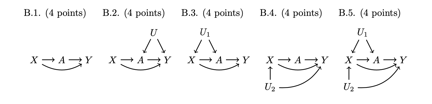
Bonus (20 points). Fun with DAGs

The bonus is required for graduate students and optional (no extra credit) for undergraduate students.

For each DAG below, answer True or False: X is a sufficient adjustment set to identify the causal effect of A on Y. Recall that X is insufficient if a backdoor path between A and Y remains unblocked conditional on X. If False, state the backdoor path that is unblocked conditional on X.