Machine learning: Regularized regression with glmnet

When predicting an outcome, it is tempting to include many predictors and their interactions. Doing so accords with two beliefs: (1) many things matter and (2) patterns may differ across population subgroups. Yet when the sample size is small, the resulting model can be highly sensitive to the particular sample used for estimation. It may not generalize well to new cases. The sample splitting lesson introduced this issue.

Regularized regression offers a way out

estimate a model with many predictors
to the degree that you are uncertain, pull the coefficient estimates toward 0

This approach yields biased estimates that are less sensitive to the training sample. It is possible that biased, low-variance estimate are better predictions than unbiased, high-variance estimates. The glmnet package supports this type of estimation. Begin by loading data.

library(tidyverse)
library(glmnet)
learning <- read_csv("learning.csv")
holdout_public <- read_csv("holdout_public.csv")

Type ?glmnet, and you will see that the function requires arguments

x a matrix of predictors
y a vector of outcome values

Create the predictor matrix and outcome vector

We can create x using the model.matrix function, which has two arguments

a model formula
- -1 excludes the intercept (because glmnet will make an intercept for us)
- g2_log_income is parent income
- g1_log_income is grandparent income
a data frame containing variables

X <- model.matrix(~ -1 + g2_log_income + g1_log_income,
                  data = learning)

We can create the outcome vector y by pulling that column (respondent income g3_log_income) from the data frame.

y <- learning$g3_log_income

Fit the model: LASSO regression

We can then fit a glmnet model.

fit <- glmnet(x = X, y = y)

By default, the model is LASSO regression, which minimize a loss function:

The loss function has two parts

squared prediction error
a penalty on large coefficients, scaled by the tuning parameter lambda

By default, glmnet estimates coefficients at a whole series of values for the penalty parameter lambda.

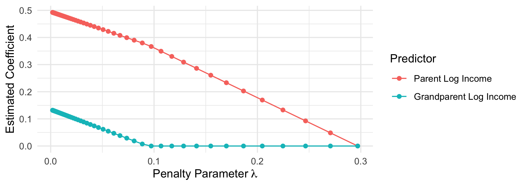
When the penalty parameter lambda is small, the prediction error dominates the loss function. At the far left, we get coefficients that are the same as we would get from OLS.

When the penalty parameter lambda is large, the penalty term dominates the loss function. At penalty parametesr above $\lambda \approx .1$ the coefficient on grandparent log income is regularized to 0—this predictor drops out of the model entirely. By $\lambda \approx .3$, both estimated coefficients are 0 and the model collapses on predicting the mean outcome for everyone.

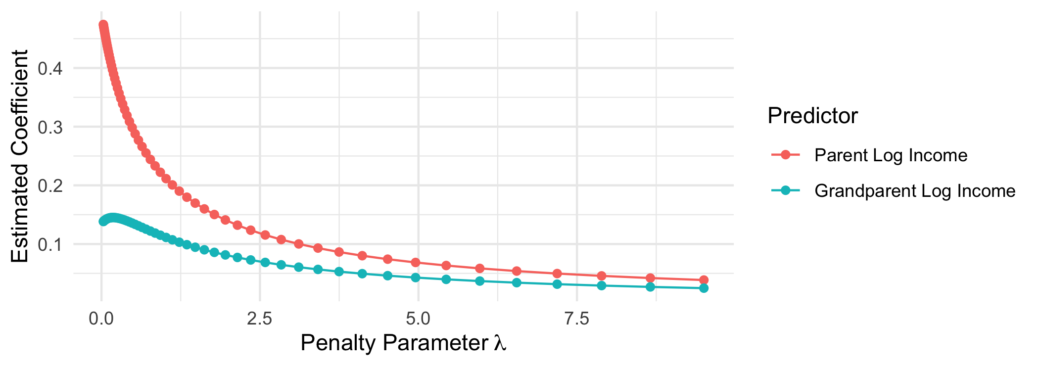
Fit the model: Ridge regression

Ridge regression is an alternative that penalizes the sum of squared coefficients.

Ridge regression heavily penalizes large coefficients: when $\beta_j$ is large, then its squared value is especially large. Ridge regression places almost no penalty on small coefficients: when $\beta_j$ is almost 0, then $\beta_j^2$ is very close to 0. For this reason, the LASSO penalty term causes some coefficents to fall to exactly 0 whereas the ridge penalty term does not.

To fit ridge regression, use the argument alpha = 0.

fit <- glmnet(x = X, y = y, alpha = 0)

This approach quickly pulls down large coefficients but never pulls coefficients exactly to zero.

Applied illustration: Many candidate predictors

Regularized regression is especially helpful in cases with many predictors. For instance, we might want to parents’ and grandparents’ incomes to interact with education, race, and sex.

formula_of_predictors <- formula(~ -1 + (g2_log_income + g1_log_income)*g3_educ*race*sex)
X <- model.matrix(formula_of_predictors,
                  data = learning)

This model has 72 predictors! With only 1365 observations, a model without regularization could be highly sensitive to the training sample and may not generalize well to out-of-sample cases.

What penalty parameter value to choose?

With glmnet, we can achieve automatic regularization. Here, we use the cv.glmnet function to automatically select the value of lambda that minimizes out-of-sample prediction error. Internally, this function uses cross validation which is a generalization of a train-test split.

fit <- cv.glmnet(x = X, y = y)

We can then use the plot() function to see the cross-validated mean squared error estimates at each penalty parameter value. We might then choose to focus on the lambda value that minimizes this prediction error.

plot(fit)

By typing coef(fit, s = "lambda.min"), you can see the estimated coefficients at the penalty parameter that minimizes cross-validated prediction error. In this case, LASSO has simplifed to 12 non-zero coefficients out of the 72 candidate predictors.

Predict for the holdout set

To predict for new cases, create a new matrix of predictors in the holdout set

X_holdout <- model.matrix(formula_of_predictors,
                          data = holdout_public)

and predict for those cases.

yhat_holdout <- predict(fit, 
                        newx = X_holdout,
                        s = "lambda.min")

If you want to put that in a data frame, note that yhat_holdout is a matrix with 1 column. You may want to extract the vector yhat_holdout[,1] to put into the holdout_public data frame.

Where to learn more

To learn more, I would recommend

Hastie, Qian, and Tay. 2021. An introduction to glmnet.